Facet-level surface energy balance in uDALES
Cities don’t have a single “surface”. A wall faces the morning sun, a south-facing roof bakes through the afternoon, and a pavement in a courtyard might never see direct light at all. uDALES resolves that geometry explicitly: every building is a triangulated surface and each triangle — a facet — carries its own energy budget through the day.
This page is a short walkthrough of what the simulation produces on the surface
side. Everything below is post-processed in Python with the udbase package
that ships with uDALES. The plots are taken straight from the official
facet tutorial notebook
— start there for the full code, helper-by-helper API, and the geometry-side
machinery (skylines, blockage ratios, building IDs) we glide over here.
Facets
A facet is one triangle of the building surface mesh. Each one knows what it
is — roof, wall, ground, or vegetation — and carries a small set of material
properties (albedo, emissivity, roughness, layer thickness, conductivity).
udbase exposes those facets directly: you can pull the full geometry into
NumPy, colour each triangle by any property or simulation output, and inspect
specific buildings.
The figure below colours every facet in a small experimental block by surface type. Drag to rotate, scroll to zoom.
Surface energy balance, face by face
For each facet at every output time, uDALES tracks the five SEB components:
- K* — net shortwave radiation absorbed at the surface, including multiple reflections between facets.
- L* — net longwave (the surface emits, neighbours and the sky emit back).
- H — turbulent sensible heat flux into the air.
- E — turbulent latent heat flux (zero for impervious surfaces).
- G — conductive heat flux into the wall or pavement, set by the layered thermal model inside each facet.
The closure K* + L* − H − E − G ≈ 0 holds per facet at every step (residuals
are a small fraction of a Watt per square metre, set by the time integration).
Per-facet quantities can be dropped onto the surface mesh for inspection. Here are two snapshots: a map of net shortwave radiation across the same block at late afternoon (note the shading from neighbouring buildings), and a map of surface temperature at the same instant.
From surfaces to a city-scale balance
The interesting question for urban climate isn’t “what’s happening on this
particular wall” but “what does the neighbourhood do as a whole”. udbase
area-averages over any selection of facets and converts back to a
projected-area basis (f = A_3D / A_2D) so the result is directly comparable
to the SEBs reported in operational weather and climate models.
Across this experiment’s diurnal cycle, the projected-area energy balance looks like:
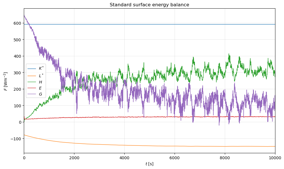
K* dominates during the day, L* is a steady night-time loss, and H and G exchange the heat between the air and the building fabric. Sidewall-only averages (selecting facets whose normal has zero z-component) tell a different story — they receive much less radiation but stay warmer overnight.
Going deeper
The full notebook covers the rest of the API: calculate_frontal_properties
for blockage ratios, assign_prop_to_fac for material lookups,
load_fac_momentum for pressure and shear, convert_facvar_to_field for
projecting facet data back onto the LES grid, and several worked examples on
sidewalls and inside-the-wall temperature profiles.
For everything beyond this overview, see the uDALES facet tutorial notebook and the uDALES repository more generally.
References
- Sützl, B. S., Rooney, G. G., & van Reeuwijk, M. (2020). Drag distribution in idealized heterogeneous urban environments. Boundary-Layer Meteorology, 178, 225–248.
- van Reeuwijk, M., & Huang, J. (2025). uDALES 2.0: a large-eddy simulation model for urban environments. Journal of Open Source Software, submitted.